
Deposit timing at the beginning or end of a month produces different balances because each beginning-of-month deposit has one extra month to earn interest. The comparison is meaningful only when the contribution amount, number of deposits, rate and final valuation date are otherwise the same.
The compound interest calculator includes an “Added at” choice for the start or end of a contribution period. This guide shows exactly what that switch means. The rates below are fictional arithmetic inputs, not offered savings rates or investment-return predictions.
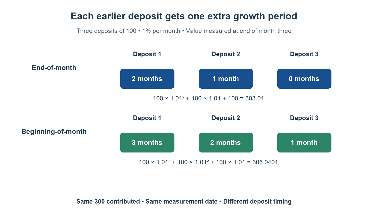
Table of Contents
Deposit timing on the same monthly timeline
Imagine a three-month period with a balance measured at the end of month three. You contribute 100 units per month, with no initial balance, at a constant 1% per month.
In the end-of-month schedule, deposits arrive at the ends of months one, two and three. The first grows for two months, the second for one month and the last has no growth period before measurement.
In the beginning-of-month schedule, deposits arrive at the starts of months one, two and three. They grow for three, two and one months respectively. Both schedules contain exactly three deposits, totalling 300 units.
Earlier deposit timing requires having the money available earlier. It is not free extra growth from an unchanged cash-flow schedule. If wages arrive only at month-end, a beginning-of-month comparison may require a cash buffer that the end-of-month plan does not.
Deposit timing example: 100 per month at 1% monthly
| Deposit number | End-of-month schedule | Beginning-of-month schedule |
|---|---|---|
| First 100 | 100 × 1.01² = 102.01 | 100 × 1.01³ = 103.0301 |
| Second 100 | 100 × 1.01 = 101.00 | 100 × 1.01² = 102.01 |
| Third 100 | 100.00 | 100 × 1.01 = 101.00 |
| Total before final display rounding | 303.01 | 306.0401 |
The end-of-month balance is 303.01; the beginning-of-month balance rounds to 306.04. The difference is about 3.03. Both plans received 300 in contributions, so the difference comes entirely from the extra time in this simplified model.
You can also check month by month. At the end of month one, the beginning schedule has 101 and the ending schedule has 100. At the end of month two, they have 203.01 and 201. At the end of month three, they have 306.0401 and 303.01.
For the deposit timing comparison, keep full precision through the calculation and round the displayed answer at the end. An actual account may apply its own daily accrual and crediting-rounding rules, so a model’s last few cents need not match a statement.
The contribution formula and the extra-period multiplier
Let C be each contribution, i the growth rate per contribution period and n the number of periods. With contributions at each period’s end:
Future value of contributions = C × ((1 + i)n − 1) ÷ i
For contributions at each period’s beginning, multiply that contribution value by (1 + i). This works because every contribution receives one extra period at the same rate.
The initial balance is separate from contribution deposit timing. If it is present at the start under both schedules, its value is P × (1 + i)n in both. Do not multiply the entire account balance by another (1 + i), because that would grant an extra period to the unchanged initial balance too.
| Periods | Total contributed | End-of-month value | Beginning-of-month value |
|---|---|---|---|
| 3 months | 300 | 303.01 | 306.04 |
| 12 months | 1,200 | 1,268.25 | 1,280.93 |
| 120 months | 12,000 | 23,003.87 | 23,233.91 |
The long example illustrates the formula, not a likely outcome. A constant 1% each month corresponds to more than 12% effective annual growth. Do not substitute a real account’s annual yield into the monthly rate field.
Reproduce the example in the calculator
Set initial principal to zero, the nominal annual rate to 12%, compounding to monthly, duration to zero years plus three months, regular contribution to 100 and contribution frequency to monthly. Compare end-of-period and start-of-period additions. In this deliberately matched model, 12% divided by 12 gives 1% per month.
Do not use this division blindly for an effective annual yield. The monthly equivalent of an effective annual rate R is (1 + R)1/12 − 1. The distinction between compounding frequencies is explored in daily vs monthly compound interest.
As an independent spreadsheet check, Excel’s FV documentation defines type 0 for period-end payments and type 1 for period-start payments. For this original example, =FV(1%,3,-100,0,0) returns 303.01, while =FV(1%,3,-100,0,1) returns 306.0401. The negative contribution follows the spreadsheet’s cash-flow sign convention.
Deposit timing checks that keep the comparison fair
- Count deposits explicitly. Including both a day-zero deposit and another at the final boundary can accidentally create n + 1 deposits.
- Use the same end date. Moving the measurement date changes every deposit’s growth time.
- Separate timing from amount. An extra contribution is not a timing benefit.
- Check rate assumptions. Variable returns, account fees, taxes, deposit limits and actual crediting dates can change results.
- Keep a usable cash buffer. A timing illustration does not decide whether locking up money earlier suits your obligations.
For the underlying growth model without a contribution-timing comparison, see how compound interest works.
Deposit timing when an initial balance is already present
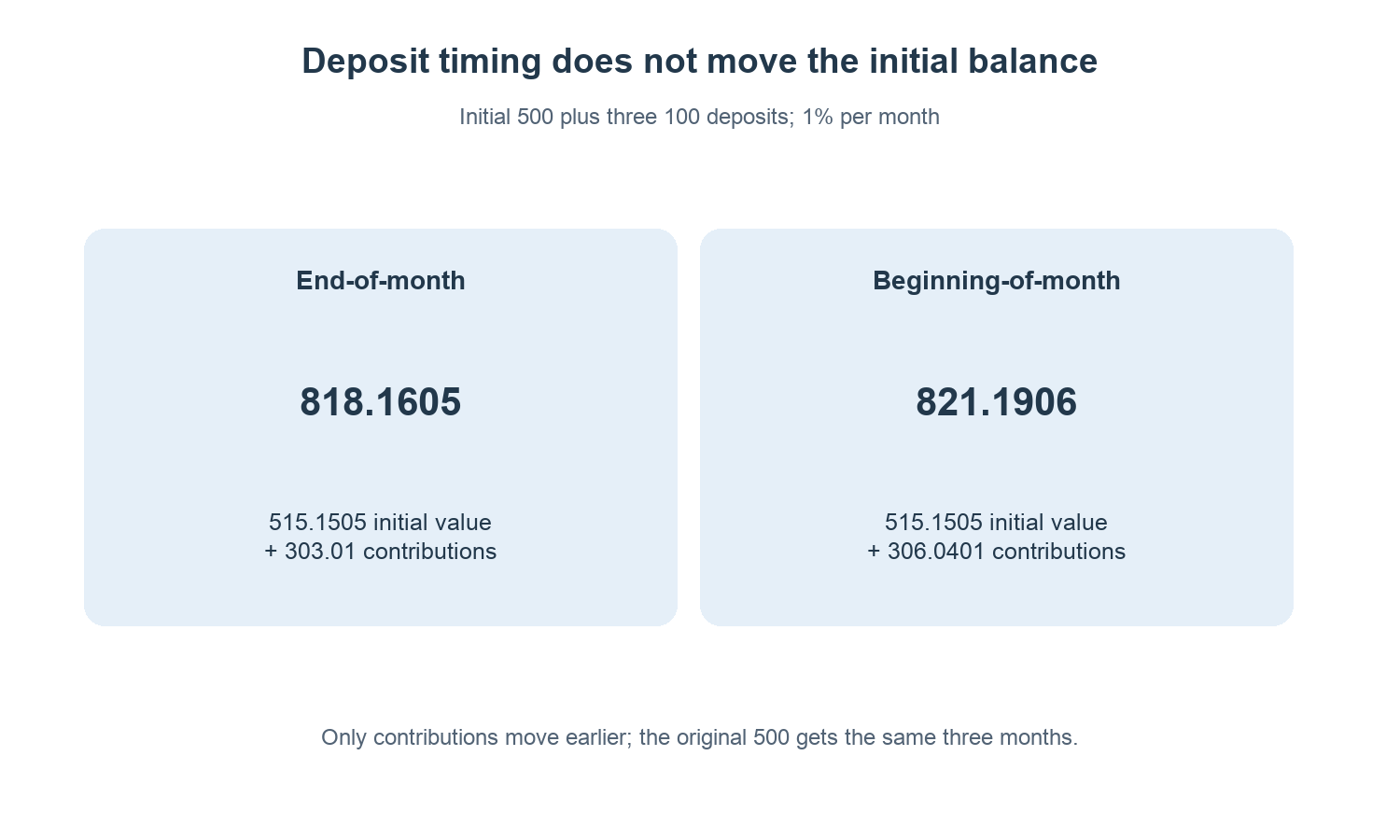
Add an initial balance of 500 to the original three-month example. That money is present from the start in both schedules. At 1% per month, its value at the end of month three is 500 × 1.01³ = 515.1505.
Add the already-calculated contribution values: the end-of-month total is 515.1505 + 303.01 = 818.1605, while the beginning-of-month total is 515.1505 + 306.0401 = 821.1906. Rounded to cents, they are 818.16 and 821.19.
| Component | End-of-month deposits | Beginning-of-month deposits |
|---|---|---|
| Future value of initial 500 | 515.1505 | 515.1505 |
| Future value of three contributions | 303.01 | 306.0401 |
| Combined balance | 818.1605 | 821.1906 |
The difference remains 3.0301 because only the contribution schedule changed. Multiplying the entire 818.1605 by 1.01 would incorrectly add another month of growth to the initial balance as well.
What if one monthly deposit is missed?
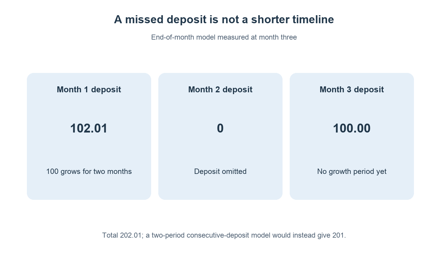
The equal-payment formula assumes a contribution every specified period. If the second end-of-month deposit is missed, the three-month schedule contains only the first 100 and the final 100. Their end value is 100 × 1.01² + 100 = 202.01.
Changing the formula’s period count from three to two would instead model two consecutive end-of-period deposits valued at the end of a two-period horizon, giving 201. That is not the same timeline. A missed contribution is a change to the cash-flow schedule, not necessarily a shorter saving horizon.
For irregular deposits, create one row for each actual contribution with its date and growth duration. The current regular-contribution controls are convenient for uniform schedules; do not present them as a transaction-by-transaction bank ledger.
Check the rate label before comparing schedules
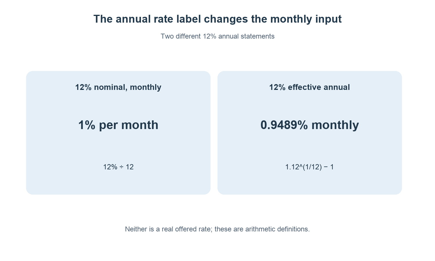
The fictional 12% nominal annual rate compounded monthly means 1% per month. Its effective annual growth is 1.01¹² − 1 ≈ 12.6825% if the balance remains invested and the assumptions hold.
By contrast, an effective annual rate of 12% corresponds to a monthly equivalent of approximately 0.9489%, since 1.121/12 − 1 ≈ 0.009489. Dividing that effective annual figure by twelve would use a different model.
Before comparing outputs, write the rate label, compounding frequency and contribution frequency beside the number. A difference attributed to deposit timing may actually come from interpreting the rate differently in the two tools.
A deposit timing comparison you can reproduce
Record the starting balance, each contribution amount, number of contributions, contribution dates or boundary convention, rate assumption and final valuation date. Then change only the timing setting while keeping the rest fixed.
Check the zero-rate case as a simple control: 500 initially plus three contributions of 100 must total 800 in either timing model when there are no fees. If the displayed contributions differ between the two schedules, inspect whether one endpoint included an extra payment.
A real account may credit interest daily, process deposits after a cutoff or restrict when a contribution starts earning. Use its terms for those details. The model demonstrates how time affects a stated calculation; it does not guarantee that sending money one calendar day earlier produces a particular credited return.
Common questions
What happens at a zero rate?
Both schedules finish with P + nC if there are no fees. The formula’s division by i needs a separate zero-rate case, but the arithmetic is simply the sum of contributions.
Does earlier always mean a higher balance?
In this constant positive-rate model, yes. That statement does not guarantee a better outcome for investments with changing or negative returns.
Is a start-of-month deposit the same as daily compounding?
No. Deposit timing determines when money enters the model. Compounding frequency determines how growth is applied. Change one setting at a time to see its separate effect.
Use the compound interest calculator to compare the two schedules while holding the other inputs constant.