
A projection of retirement contributions in today’s dollars can still be inconsistent even when its return formula is correct. A fixed cash contribution of $1,200 each future year is not the same as contributing $1,200 of today’s purchasing power each year. The second promise requires larger cash payments if prices rise.
This worksheet audits those contribution assumptions with a short three-year example. It complements our guide to inflation and retirement calculators, which explains nominal and real returns. The task here is to make every payment and balance use a stated date and unit.
The Retirement Calculator uses nominal returns and a separate inflation input. Its annual contribution increase is a separate assumption. Entering inflation does not automatically promise that your cash retirement contributions will rise at that rate.
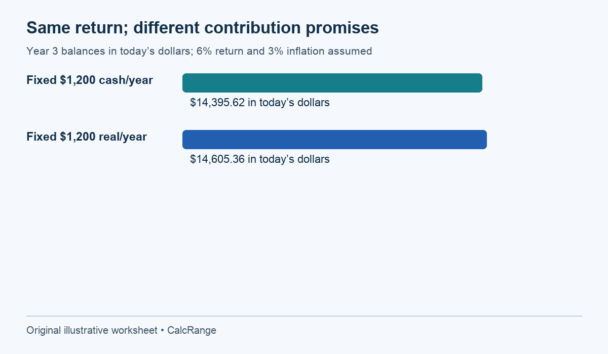
Table of Contents
Write a dated retirement contributions ledger
Assume $10,000 invested today, a hypothetical 6% annual nominal return and 3% annual inflation. Ignore fees and taxes in this small arithmetic example. Contributions arrive at the end of each year, after that year’s growth. These are teaching assumptions, not forecasts or investment recommendations.
The U.S. Bureau of Labor Statistics explains nominal and real amounts by distinguishing currency values from values adjusted for price changes. Our assumed 3% is not a quoted current CPI rate, and one national price index does not precisely describe every household’s spending.
For this example, the price index starts at 1.000 today, then becomes 1.030, 1.0609 and 1.092727. Divide a future balance by that year’s index to express it in today’s dollars. Do not divide all three balances by the final year’s index.
Scenario A: fixed cash retirement contributions of $1,200 each year
At the end of year one, the original $10,000 grows to $10,600; adding $1,200 gives $11,800. Year two becomes $11,800 × 1.06 + $1,200 = $13,708. The year-three balance is $15,730.48.
| Year end | Cash contribution | Nominal balance | Balance in today’s dollars |
|---|---|---|---|
| 1 | $1,200.00 | $11,800.00 | $11,456.31 |
| 2 | $1,200.00 | $13,708.00 | $12,921.10 |
| 3 | $1,200.00 | $15,730.48 | $14,395.62 |
The payment is unchanged on the bank statement, but its purchasing power declines. The third $1,200 contribution is $1,200 ÷ 1.092727, approximately $1,098.17 in today’s dollars. A real-money model must reflect that shrinking contribution, not keep adding a constant real $1,200.
Scenario B: retirement contributions of $1,200 in today’s purchasing power
Now assume the goal is a constant real contribution, payable at each year-end. The cash payments must rise with the index: $1,236 in year one, $1,273.08 in year two and $1,311.2724 in year three before currency rounding.
Notice that the first future payment is already inflation-adjusted. Starting with $1,200 at the end of year one and raising it 3% afterward describes a different baseline. It preserves the first payment’s year-one purchasing power, rather than making that first payment worth $1,200 today.
| Year end | Cash contribution | Nominal balance | Balance in today’s dollars |
|---|---|---|---|
| 1 | $1,236.00 | $11,836.00 | $11,491.26 |
| 2 | $1,273.08 | $13,819.24 | $13,025.96 |
| 3 | $1,311.27 displayed | $15,959.67 | $14,605.36 |
The underlying calculation retains precision; displayed money is rounded to cents. Scenario B ends about $209.74 higher in today’s purchasing power than scenario A. The difference comes from larger contributions and their growth, not from a better investment return.
Reconcile retirement contributions in real and nominal models
The exact real annual return is (1.06 ÷ 1.03) − 1, approximately 2.912621%. For scenario B, multiply the real starting balance by 1.02912621 each year and add a real $1,200 at year-end. This reproduces the real balances in the second table.
For scenario A, use that same real return but add $1,200 ÷ 1.03 in year one, $1,200 ÷ 1.0609 in year two and $1,200 ÷ 1.092727 in year three. A fixed nominal contribution becomes a declining real contribution. Both conventions reconcile when each cash flow is converted at its own date.
This is a useful spreadsheet check: the nominal year-three balance divided by the year-three price index should equal the real-model balance, allowing only displayed rounding differences. If not, inspect payment timing and contribution escalation before changing the assumed return.
Map retirement contributions to the calculator carefully
In CalcRange, enter a nominal return before investment fees, inflation separately and fees in their own field. Enter the retirement spending goal in today’s money; the tool inflates it to the retirement date. Its projected and required funds are amounts at retirement, so compare them on that same basis.
The annual contribution increase field describes how payments change. Use 0% for a fixed cash contribution scenario. A 3% annual increase is a separate cash-flow assumption that may approximate inflation-linked saving under a 3% inflation scenario, but confirm the first payment’s timing and base amount.
The hand-worked tables here use one contribution at each year-end, whereas the calculator accepts monthly contributions. Do not expect its balance to match these annual-payment tables exactly. The worksheet tests consistency of assumptions; it is not a claim that the tool uses this simplified annual schedule.
Employer contributions, a future lump sum and pension growth are separate inputs. A fixed future lump sum should not be silently treated as a present-value amount. Write when the money arrives and whether its stated value is in current or future currency before entering it.
Three retirement contributions checks for a longer projection
A future spending target is not an extra inflation adjustment to returns
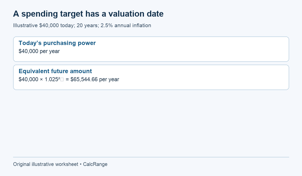
Assume an annual spending goal of $40,000 in today’s purchasing power, a 20-year horizon and hypothetical 2.5% annual inflation. The equivalent annual amount at year 20 is $40,000 × 1.025²⁰, approximately $65,544.66. These are two descriptions of the same assumed spending power at different dates.
If a calculator asks for today’s spending and applies inflation internally, enter $40,000. Entering $65,544.66 into that same field would inflate the already inflated amount again. The resulting target would describe more spending power than intended, even if every formula executes correctly.
Conversely, a tool that explicitly asks for a future-dollar target may require the larger number. Read the field label and method. Keep a note stating “today’s amount” or “amount at retirement” rather than relying on the currency symbol alone. A dollar sign does not encode its valuation date.
A lump sum provides an independent conversion check
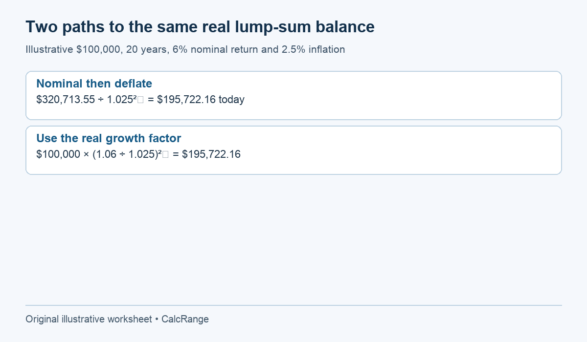
Start with $100,000, assume 6% nominal growth for 20 years and make no contributions or withdrawals. The nominal future balance is $100,000 × 1.06²⁰, approximately $320,713.55. At the same hypothetical 2.5% inflation rate, divide by 1.025²⁰ to obtain about $195,722.16 in today’s dollars.
The exact real growth factor is 1.06 ÷ 1.025. Therefore $100,000 × (1.06 ÷ 1.025)²⁰ gives the same $195,722.16. This is a useful two-path identity test because no contribution timing is involved. If these paths disagree materially, the conversion or rounding is inconsistent.
These assumed growth rates are constant for teaching purposes. Actual returns and prices vary. The example verifies algebra, not a likely investment outcome or a recommendation to choose a particular return assumption.
Fees and contribution growth need their own labels
Suppose one saved projection uses a nominal return before fees and another uses an expected return already reduced for fees. If both also subtract a fee input, the second may count that cost twice. Before comparing balances, identify whether the quoted return assumption is gross or net of the modeled fee.
The same check applies to contribution escalation. A promise to raise deposits by 3% each year is a plan about future cash flows. It is not guaranteed merely because inflation is set to 3%, and it may be difficult to sustain if income changes. Compare a fixed-deposit scenario and an increasing-deposit scenario as separate choices.
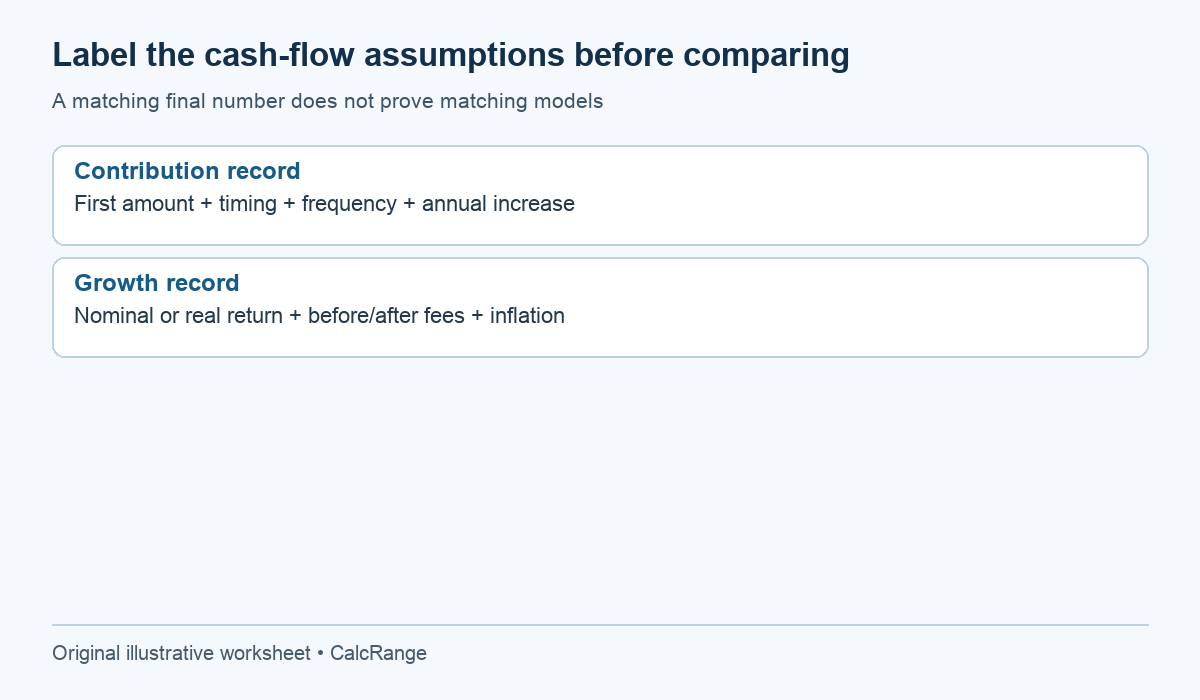
For every scenario, retain a short input card: starting savings, first contribution amount, payment frequency, first payment date, escalation rule, return basis, inflation and fees. This card often explains a difference between calculators more clearly than inspecting only their final balances.
When a tool’s conventions are not documented, label the comparison as unresolved rather than adjusting assumptions until the totals happen to agree. Two different cash-flow models can produce the same final number by coincidence. Matching the number is less important than matching the meaning of each input and output.
For a reproducible handover, add a period column to the contribution ledger. A payment recorded at the end of year one grows for two further years in this three-year example; a payment at the end of year three does not receive another year of return inside that horizon. Moving the same payment to the beginning of a year changes its exposure to growth. Record the timing before comparing calculator totals, and do not explain a timing mismatch by changing the assumed return until the answers happen to agree.
Audit two projections before comparing their totals
- Are both balances measured at the same retirement date?
- Are both expressed in today’s dollars or both in future dollars?
- Do contributions begin at the same time and rise by the same rule?
- Are returns nominal before fees, nominal after fees or real?
- Are taxes, other income and withdrawals treated consistently?
A higher displayed fund can reflect a different unit or larger assumed deposits rather than an improved plan. Keep a small assumption log with each saved result. Use the retirement target guide for spending and withdrawal assumptions, then test alternatives without interpreting a deterministic balance or readiness percentage as a probability of success.